The banking and finance industry has been one of the biggest beneficiaries of digital advancements. Many technological innovations find practical applications in finance, providing convenience and efficiency that can set institutions apart in a competitive market. However, this ease and accessibility have also led to increased fraud, particularly in credit card transactions, which remain a growing concern for consumers and financial institutions.
Traditional fraud detection systems rely on rule-based methods that struggle in real-time scenarios. These outdated approaches are often reactive, identifying fraud only after it occurs. Without real-time capabilities or advanced reasoning, they fail to match fraudsters’ rapidly evolving tactics. A more proactive and sophisticated solution is essential to combat this threat effectively.
This is where graph analytics and real-time stream processing come into play. Combining PuppyGraph, the first and only graph query engine, with DeltaStream, a stream processing engine powered by Apache Flink, enables institutions to improve fraud detection accuracy and efficiency, including real-time capabilities. In this blog post, we’ll explore the challenges of modern fraud detection and the advantages of using graph analytics and real-time processing. We will also provide a step-by-step guide to building a fraud detection system with PuppyGraph and DeltaStream.
Let’s start by examining the challenges of modern fraud detection.
Common Fraud Detection Challenges
Credit card fraud has always been a game of cat and mouse. Even before the rise of digital processing and online transactions, fraudsters found ways to exploit vulnerabilities. With the widespread adoption of technology, fraud has only intensified, creating a constantly evolving fraud landscape that is increasingly difficult to navigate. Key challenges in modern fraud detection include:
- Volume: Daily credit card transactions are too vast to review and identify suspicious activity manually. Automation is critical to sorting through all that data and identifying anomalies.
- Complexities: Fraudulent activity often involves complex patterns and relationships that traditional rule-based systems can’t detect. For example, fraudsters may use stolen credit card information to make a series of small transactions before a large one or use multiple cards in different locations in a short period.
- Real-time: The sooner fraud is detected, the less financial loss there will be. Real-time analysis is crucial in detecting and preventing transactions as they happen, especially when fraud can be committed at scale in seconds.
- Agility: Fraudsters will adapt to new security measures. Fraud detection systems must be agile, even learning as they go, to keep up with the evolving threats and tactics.
- False positives: While catching fraudulent transactions is essential, it’s equally important to avoid flagging legitimate transactions as fraud. False positives can frustrate customers, especially when a card is automatically locked out due to legitimate purchases. As a consequence, they can adversely affect revenue.
To tackle these challenges, businesses require a solution that processes large volumes of data in real-time, identifies complex patterns, and evolves with new fraud tactics. Graph analytics and real-time stream processing are essential components of such a system. By mapping and analyzing transaction networks, businesses can more effectively detect anomalies in customer behavior and identify potentially fraudulent transactions.
Leveraging Graph Analytics for Fraud Detection
Traditional fraud detection methods analyze individual transactions in isolation. This can miss connections and patterns that emerge when we examine the bigger picture. Graph analytics allows us to visualize and analyze transactions as a network of connected things.
Think of it like a social network. Each customer, credit card, merchant, and device becomes a node in the graph, and each transaction connects those nodes. We can find hidden patterns and anomalies that indicate fraud by looking at the relationships between nodes.
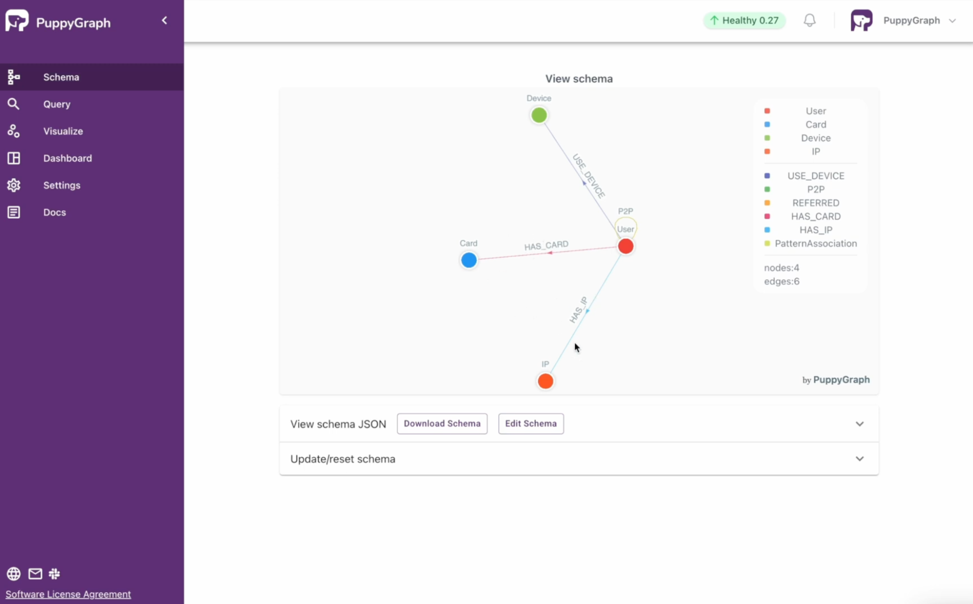
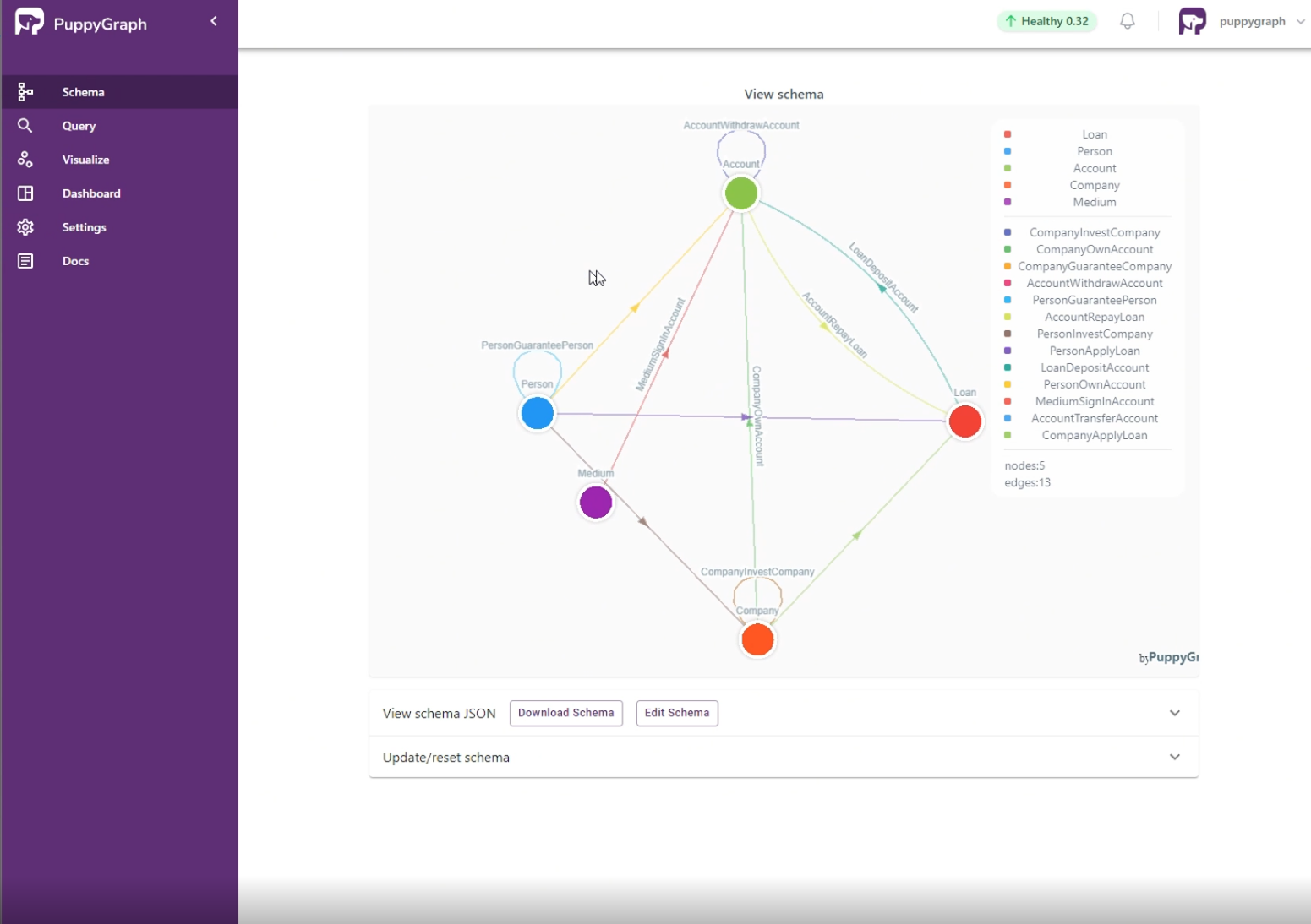
Figure: an example schema for fraud detection use case
Here’s how graph analytics can be applied to fraud detection:
- Finding suspicious connections: Graph algorithms can discover unusual patterns of connections between entities. For example, if the same person uses multiple credit cards in different locations in a short period or a single card is used to buy from a group of merchants known for fraud, those connections will appear in the graph and be flagged as suspicious.
- Uncovering fraud rings: Fraudsters often work within the same circles, using multiple identities and accounts to carry out scams. Graph analytics can find those complex networks of people and their connections, helping to identify and potentially break up entire fraud rings.
- Surfacing identity theft: When a stolen credit card is used, the spending patterns will generally be quite different from the cardholder’s normal behavior. By looking at the historical and current transactions within a graph, you can see sudden changes in spending habits, locations, and types of purchases that may indicate identity theft.
- Predicting future fraud: Graph analytics can predict future fraud by looking at historical data and the patterns that precede a fraudulent transaction. By predicting fraud before it happens, businesses can take action to prevent it.
Of course, all of these benefits are extremely helpful. However, the biggest hurdle to realizing them is the complexity of implementing a graph database. Let’s look at some of those challenges and how PuppyGraph can help users avoid them entirely.
Challenges of Implementing and Running Graph Databases
As shown, graph databases can be an excellent tool for fraud detection. So why aren’t they used more frequently? This usually boils down to implementing and managing them, which can be complex for those unfamiliar with the technology. The hurdles that come with implementing a graph database can far outweigh the benefits for some businesses, even stopping them from adopting this technology altogether. Here are some of the issues generally faced by companies implementing graph databases:
- Cost: Traditional relational databases have been the norm for decades, and many organizations have invested heavily in their infrastructure. Switching to a graph database or even running a proof of concept requires a significant upfront investment in new software, hardware, and training.
- Implementing ETL: Extracting, transforming, and loading (ETL) data into a graph database can be tricky and time-consuming. Data needs to be restructured to fit into a graph model, which requires knowledge of the underlying data to be moved over and how to represent these entities and relationships within a graph model. This requires specific skills and adds to the implementation time and cost, meaning the benefits may be delayed.
- Bridging the skills gap: Graph databases require a different data modeling and querying approach from traditional databases. In addition to the previous point regarding ETL, finding people with the skills to manage, maintain, and query the data within a graph database can also be challenging. Without these skills, graph technology adoption is mostly dead in the water.
- Integration challenges: Integrating a graph database with existing systems and applications is complex. This usually involves taking the output from graph queries and mapping them into downstream systems, which requires careful planning and execution. Getting data to flow smoothly and be compatible with different systems is significant.
These challenges highlight the need for solutions that make graph database adoption and management more accessible. A graph query engine like PuppyGraph addresses these issues by enabling teams to integrate their data and query it as a graph in minutes without the complexity of ETL processes or the need to set up a traditional graph database. Let’s look at how PuppyGraph helps teams become graph-enabled without ETL or the need for a graph database.
How PuppyGraph Solves Graph Database Challenges
PuppyGraph is built to tackle the challenges that often hinder graph database adoption. By rethinking graph analytics, PuppyGraph removes many entry barriers, opening up graph capabilities to more teams than otherwise possible. Here’s how PuppyGraph addresses many of the hurdles mentioned above:
- Zero-ETL: One of PuppyGraph’s most significant advantages is connecting directly to your existing data warehouses and data lakes—no more complex and time-consuming ETL. There is no need to restructure data or create separate graph databases. Simply connect the graph query engine directly to your SQL data store and start querying your data as a graph in minutes.
- Cost: PuppyGraph reduces the expenses of graph analytics by using your existing data infrastructure. There is no need to invest in new database infrastructure or software and no ongoing maintenance costs of traditional graph databases. Eliminating the ETL process significantly reduces the engineering effort required to build and maintain fragile data pipelines, saving time and resources.
- Reduced learning curve: Traditional graph databases often require users to master complex graph query languages for every operation, including basic data manipulation. PuppyGraph simplifies this by functioning as a graph query engine that operates alongside your existing SQL query engine using the same data. You can continue using familiar SQL tools for data preparation, aggregation, and management. When more complex queries suited to graph analytics arise, PuppyGraph handles them seamlessly. This approach saves time and allows teams to reserve graph query languages specifically for graph traversal tasks, reducing the learning curve and broadening access to graph analytics.
- Multi-query language support: Engineers can continue to use their existing SQL skills and platform, allowing them to leverage graph querying when needed. The platform offers many ways to build graph queries, including Gremlin and Cypher support, so your existing team can quickly adopt and use graph technology.
- Effortless scaling: PuppyGraph’s architecture separates compute and storage so it can easily handle petabytes of data. By leveraging their underlying SQL storage, teams can effortlessly scale their compute as required. You can focus on extracting value from your data without scaling headaches.
- Fast deployment: With PuppyGraph, you can deploy and start querying your data as a graph in 10 minutes. There are no long setup processes or complex configurations. Fast deployment means you can start seeing the benefits of graph analytics and speed up your fraud detection.
In short, PuppyGraph removes the traditional barriers to graph adoption so more institutions can use graph analytics for fraud detection use cases. By simplifying, reducing costs, and empowering existing teams with effortless graph adoption, PuppyGraph makes graph technology accessible for all teams and organizations.
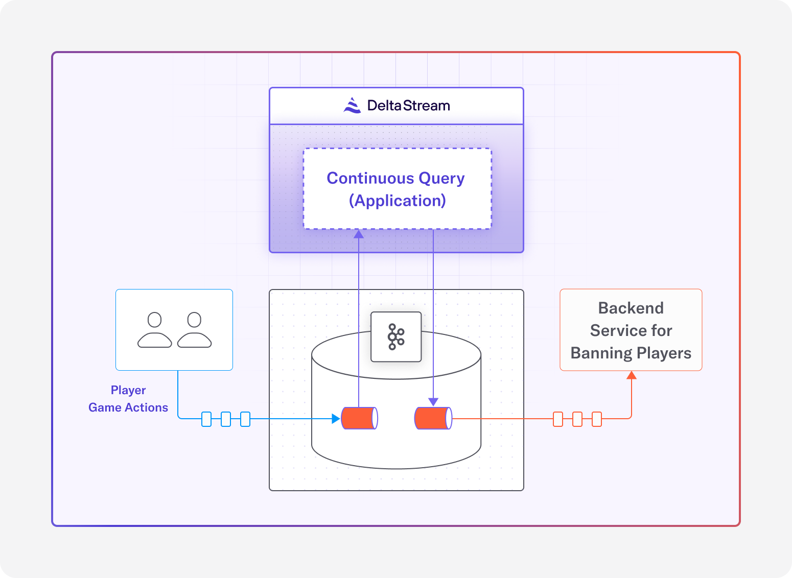
Real-Time Fraud Prevention with DeltaStream
Speed is key in the fight against fraud, and responsiveness is crucial to preventing or minimizing the impact of an attack. Systems and processes that act on events with minimal latency can mean the difference between successful and unsuccessful cyber attacks. DeltaStream empowers businesses to analyze and respond to suspicious transactions in real-time, minimizing losses and preventing further damage.
Why Real-Time Matters:
- Immediate Response: Rapid incident response means security and data teams can detect, isolate, and trigger mitigation protocols, minimizing their vulnerability window faster than ever. With real-time data and sub-second latency, the Mean Time to Detect (MTTD) and Mean Time to Respond (MTTR) can be significantly reduced.
- Proactive Prevention: Data and security teams can identify behavior patterns as they emerge and implement mitigation tactics. Real-time allows for continuous monitoring of system health and security with predictive models.
- Improved Accuracy: Real-time data provides a more accurate view of customer behavior for precise detection. Threats are more complex than ever and often involve multi-stage attack patterns; streaming data aids in identifying these complex and ever-evolving threat tactics.
DeltaStream’s Key Features:
- Speed: Increase the speed of your data processing and your team’s ability to create data applications. Reduce latency and cost by shifting your data transformations out of your warehouse and into DeltaStream. Data teams can also quickly write queries in SQL to create analytics pipelines with no other complex languages to learn.
- Team Focus: Eliminate maintenance tasks with our continually optimizing Flink operator. Your team isn’t focused on infrastructure, meaning they can focus on building and strengthening pipelines.
- Unified View: An organization’s data rarely comes from just one source. Process streaming data from multiple sources in real-time to get a complete picture of activities. This means transaction data, user behavior, and other relevant signals can be analyzed together as they occur.
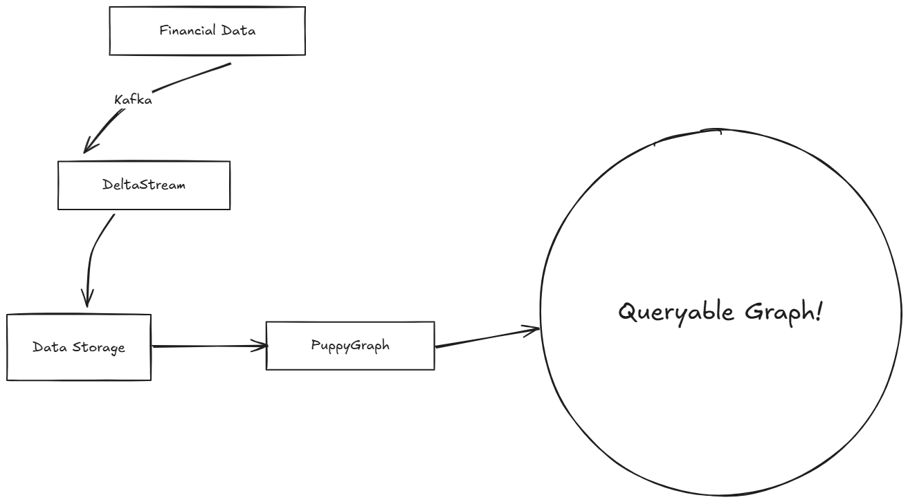
By combining PuppyGraph’s graph analytics with DeltaStream’s real-time processing, businesses can create a dynamic fraud detection system that stays ahead of evolving threats.
Step-by-Step tutorial: DeltaStream and PuppyGraph
In this tutorial, we go through the high-level steps of integrating DeltaStream and PuppyGraph.
The detailed steps are available at:
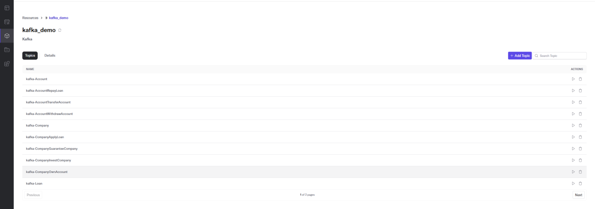
Starting a Kafka Cluster
We start a Kafka Server as the data input. (Later in the tutorial, we’ll send financial data through Kafka.)
We create topics for financial data like this:
bin/kafka-topics.sh --create --topic kafka-Account --bootstrap-server localhost:9092 --partitions 1 --replication-factor 1
Setting up DeltaStream
Connecting to Kafka
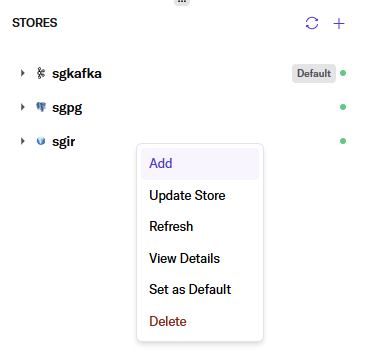
Log in to the Deltastream console. Then, navigate to Resources and add a Kafka Store – for example, kafka_demo – with the Kafka Cluster parameters we created in the previous step.
Next, in the Workspace, create a deltastream database – for example: kafka_db
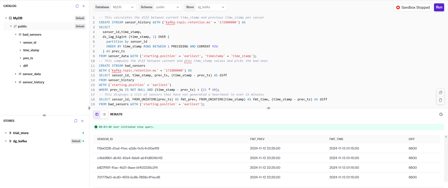
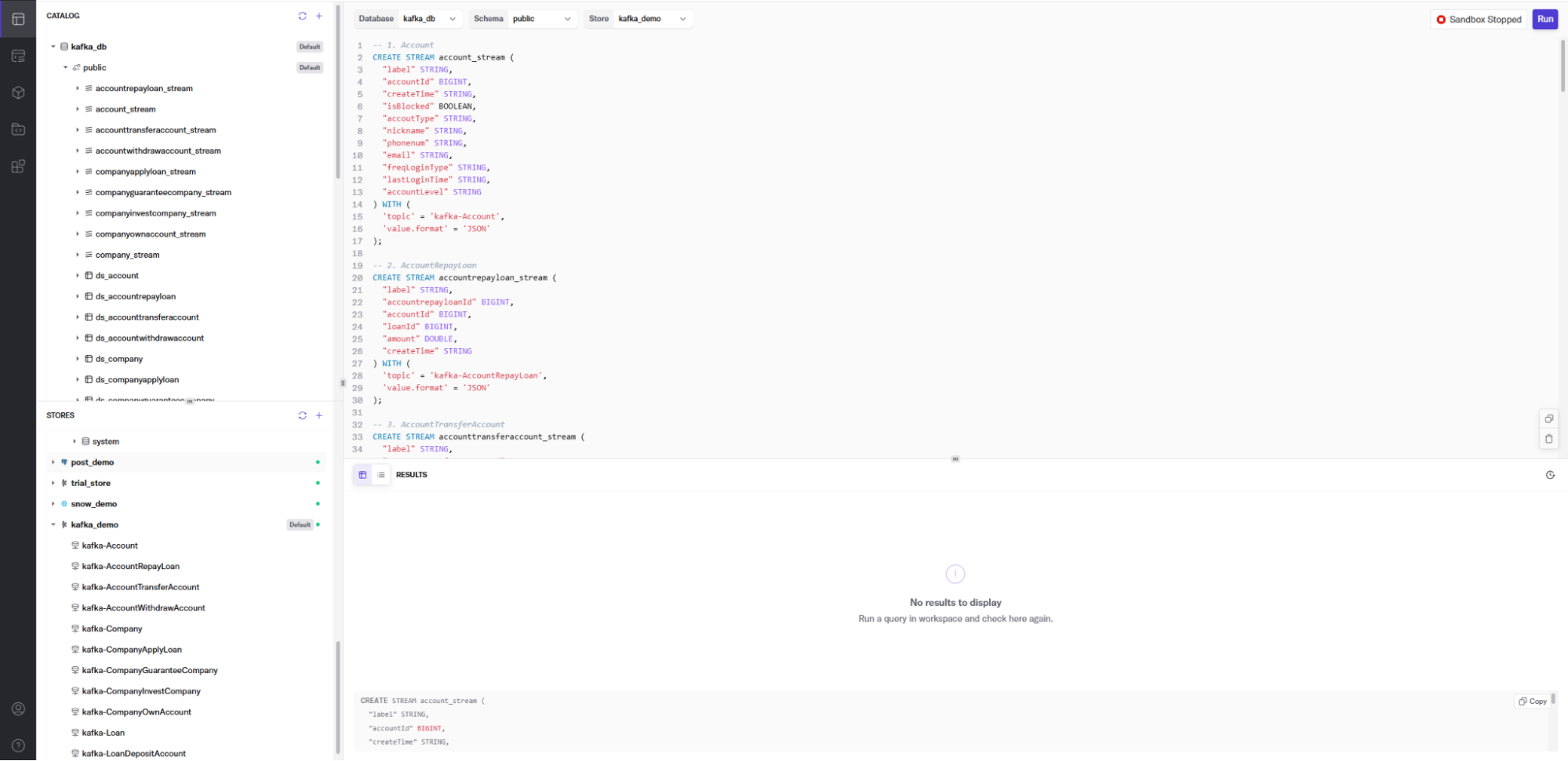
After that, we use DeltaStream SQL to create streams for the Kafka topics we created in the previous step. The stream describes the topic’s physical layout so it can be easily referenced with SQL. Here is an example of one of the streams we create in DeltaStream for a Kafka topic. Once we declare the streams, we can build streaming data pipelines to transform, enrich, aggregate, and prepare streaming data for analysis in PuppyGraph. First, we’ll define the account_stream from the kafka-Account topic.
CREATE STREAM account_stream (
"label" STRING,
"accountId" BIGINT,
"createTime" STRING,
"isBlocked" BOOLEAN,
"accoutType" STRING,
"nickname" STRING,
"phonenum" STRING,
"email" STRING,
"freqLoginType" STRING,
"lastLoginTime" STRING,
"accountLevel" STRING
) WITH (
'topic' = 'kafka-Account',
'value.format' = 'JSON'
);
Next, we’ll define the accountrepayloan_stream from the kafka-AccountRepayLoan topic:
CREATE STREAM accountrepayloan_stream (
"label" STRING,
"accountrepayloandid" BIGINT,
"loanId" BIGINT,
"amount" DOUBLE,
"createTime" STRING
) WITH (
'topic' = 'kafka-AccountRepayLoan',
'value.format' = 'JSON'
);
And finally, we’ll show the accounttransferaccount_stream from the kafka-AccountTransferAccount. You’ll note there is both a fromid and toid that will like to the loanId. This allows us to enrich data in the account payment stream with account information from the account_stream and combine it with the account transfer stream.
With DeltaStream, this can then easily be written out as a more succinct and enriched stream of data to our destination, such as Snowflake or Databricks. We combine data from three streams with just the information we want, preparing the data in real-time from multiple streaming sources, which we then graph using PuppyGraph.
CREATE STREAM accounttransferaccount_stream (
"label" VARCHAR,
"accounttransferaccountid", BIGINT,
"fromd" BIGINT,
"toid" BIGINT,
"amount" DOUBLE,
"createTime" STRING,
"ordernum" BIGINT,
"comment" VARCHAR,
"paytype" VARCHAR,
"goodstype" VARCHAR
) WITH (
'topic' = 'kafka-AccountTransferAccount',
'value.format' = 'JSON'
);
Adding a Store for Integration
PuppyGraph will connect to the stores and allow querying as a graph.
Once our data is ready in the desired format, we can write streaming SQL queries in DeltaStream to write data continuously in the desired storage. In this case, we can use DeltaStream’s native integration with Snowflake or Databricks, where we will use PoppyGraph. Here is an example of writing data continuously into a table in Snowflake or Databricks from DeltaStream:
CREATE TABLE ds_account
WITH
(
'store' = '<store_name>'
<Storage parameters>
) AS
SELECT * FROM account_stream;
Starting data processing
Now, you can start a Kafka Producer to send the financial JSON data to Kafka. For example, to send account data, run:
kafka-console-producer.sh --broker-list localhost:9092 --topic kafka-Account < json_data/Account.json
DeltaStream will process the data, and then we will query it as a graph.
Query your data as a graph
You can start PuppyGraph using Docker. Then upload the Graph schema, and that’s it! You can now query the financial data as a graph as DeltaStream processes it.
Start PuppyGraph using the following command:
docker run -p 8081:8081 -p 8182:8182 -p 7687:7687 \
-e DATAACCESS_DATA_CACHE_STRATEGY=adaptive \
-e <STORAGE PARAMETERS> \
--name puppy --rm -itd puppygraph/puppygraph:stable
Log into the PuppyGraph Web UI at http://localhost:8081 with the following credentials:
Username: puppygraph
Password: puppygraph123
Upload the schema:Select the file schema_<storage>.json in the Upload Graph Schema JSON section and click Upload.
Navigate to the Query panel on the left side. The Gremlin Query tab offers an interactive environment for querying the graph using Gremlin. For example, to query the accounts owned by a specific company and the transaction records of these accounts, you can run:
g.V("Company[237]")
.outE('CompanyOwnAccount').inV()
.outE('AccountTransferAccount').inV()
.path()
Conclusion
As this blog post explores, traditional fraud detection methods simply can’t keep pace with today’s sophisticated criminals. Real-time analysis and the ability to identify complex patterns are critical. By combining the power of graph analytics with real-time stream processing, businesses can gain a significant advantage against fraudsters.
PuppyGraph and DeltaStream offer robust and accessible solutions for building real-time dynamic fraud detection systems. We’ve seen how PuppyGraph unlocks hidden relationships and how DeltaStream analyzes real-time data to quickly and accurately identify and prevent fraudulent activity. Ready to take control and build a future-proof, graph-enabled fraud detection system? Try PuppyGraph and DeltaStream today. Visit PuppyGraph and DeltaStream to get started!