13 May 2025
Min Read
Medical IOT Data with Kafka and Iceberg
Have you ever spent time in the hospital or had biometric tests done? Those devices generate and save a lot of information that should prompt some action or process. We often look for anomalies in alert situations, but there are significantly more uses for that data. You might be wearing a heart monitor to record information for a possible procedure or a sleep study that records your vitals to identify a problem. These devices are constantly improving their ability to collect actionable information and improve our lives.
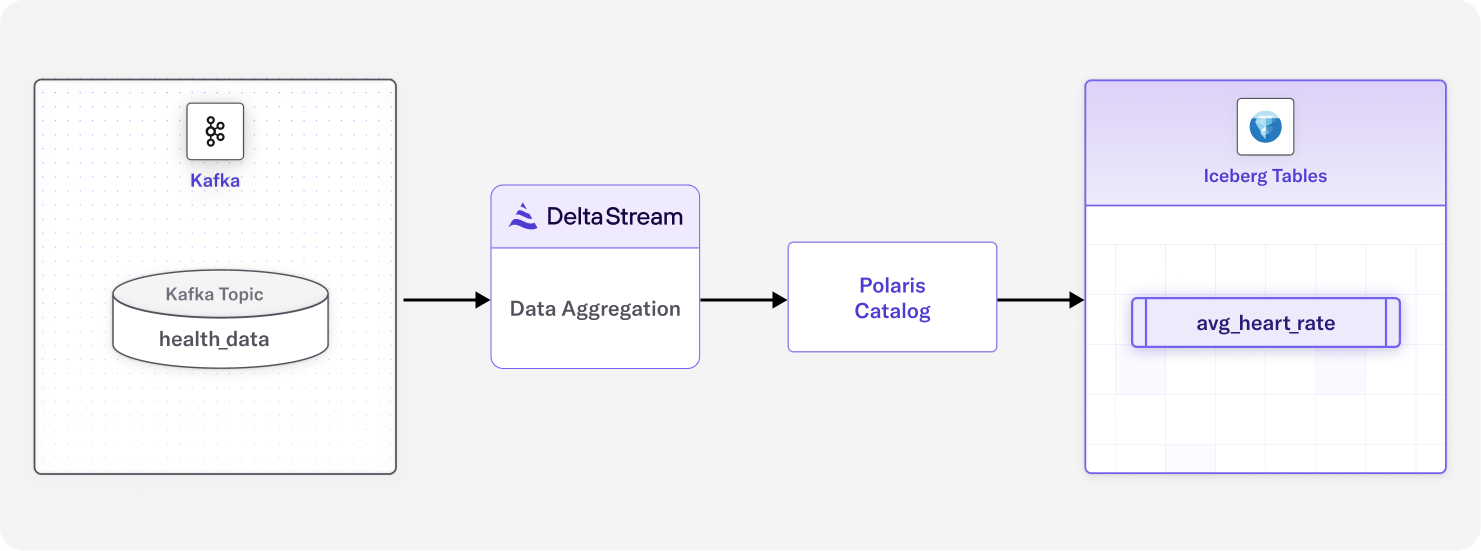
DeltaStream provides a powerful ability to process data in Apache Kafka topics and write to various destinations, including Apache Iceberg. The AWS Glue and Apache Polaris (incubating) catalogs are supported. For this example, we’ll be using Polaris. If you are unfamiliar with DeltaStream, this short interactive demo will walk you through it. With that out of the way, let’s look at our setup.
Use Case: Aggregating IOT Data to Iceberg
For this example, we’ll use a stream of simulated data containing a timestamp, patient ID, and assorted vital information. The description will be in the solution section. The data stream will be aggregated into a new table written to Iceberg, which will be our source of truth.
Our data is comprised of the following:
- Inbound health_data Kafka topic with the following data:
- 100 patients
- Sensor data emitted every 10 minutes for 6 months starting June 1, 2024
- Sensor data fields are randomly generated between normal bounds for the fields
- Outbound to Iceberg aggregated patient and heart rate data
Our queries do the following:
- Aggregate the hourly average heart rate per patient from Kafka and write to Iceberg
- Find the top 3 patients with the highest daily heart rate for each month
Setup and Solution
First, let’s define the data we are working with. Our Kafka topic health_data looks like this:
That means we need to create a DeltaStream Stream-type Object. We do this with a CSAS statement:
Our next step is to create an Iceberg table to hold our hourly average heart rate data. The following CTAS does that for us, and this is where the magic happens. We can aggregate our data in flight before we land it in Iceberg. This dramatically reduces latency, eliminates compute costs for transformation, and reduces storage size. If you are unfamiliar with configuring Iceberg in DeltaStream, this short interactive demo can walk you through it.
Our resulting data looks like this:
Now that we have an Iceberg table with our patient ID, the average hourly heart rate, and the time window, we can look at the patients with the highest heart rate in a given month. DeltaStream enables us to immediately perform analytics on the data it just processed from Kafka to Iceberg without leaving the DeltaStream environment or performing any additional configurations – using only familiar SQL.
This query can look daunting, but it’s not a lot of code for some powerful results. Let’s break it down.
Step 1: Creating a Common Table Expression (CTE)
The query begins with a CTE named ranked_heart_rates. This temporary result set performs the initial data preparation and ranking.
Step 2: Extracting Time Components
We extract the month and year from the window_start timestamp, creating separate columns for easier grouping and sorting using DeltaStream Temporal Functions:
Step 3: Ranking Records with Window Functions
The heart of this query uses the ROW_NUMBER() window function to assign a rank to each patient's heart rate within its month-year group:
This function:
- PARTITION BY divides the data into month-year segments
- ORDER BY avg_hr DESC ranks records with highest heart rates first
- The window frame specification ensures proper calculation across the partition
Step 4: Filtering for Valid Time Windows
We only include records where the start and end timestamps fall within the same calendar month and year. Our sample data is all in 2024, but this takes into account crossing the year boundary:
Step 5: Selecting the Top 3 Per Month
Finally, the main query filters the ranked results only to include the top 3 entries per month and orders them chronologically:
Processing Medical Device Data
We just walked through a scenario for processing medical device data coming in via a Kafka topic by consolidating average hourly data per patient and writing it to Iceberg. We then immediately queried the data in Iceberg from DeltaStream to find patients with the highest average heart rate per month. A visualization tool could be used on that same Iceberg data, further taking advantage of open table formats. Notably, we performed a “shift-left” with our processing. We were able to aggregate data in flight. Then we landed that data in Iceberg, thus reducing latency and additional storage and compute costs, seamlessly preparing the data for usage in a single place.